Cumsum and Diff Tricks
There are many instances where you want to look for “trigger” events in a table (data frame) that mark the beginning of a sequence of records that need to be grouped together. While in some cases the end of such a sequence may be defined by the next similar event, in some cases there may be different “trigger” event values that mark the end of such a group of records.
For example, we might have records of wind direction and be interested in identifying periods when the direction was generally toward the west. The beginning of such a period would be a record for which the direction is “west”, but the direction in the previous record was something other than “west”. Such a period of westerly wind direction would logically end when the direction again became something other than “west”.
The obvious solution for automating the identification of such groups of records is to write a while or for loop that sequentially examines each record and uses if-else logic to generate a new column in the table that indicates the assignment of each record to an appropriate group. However, in many (but not all) cases such logic can instead be implemented using fast-running vectorized functions by creating a sequence of a few column-wise vectors that lead to generation of such a grouping column using simpler and faster basic operations.
(Note that these techniques can be applied in Python as well, using numpy/pandas functions, but examples in Python are not included in this post.)
suppressPackageStartupMessages({
  library(dplyr)
  library(ggplot2)
  library(kableExtra)
})
theme_set(theme_minimal())
The idea
If we have a timeline, or any real number line, we may be able to figure out when certain things happened, but it may be useful to lump records following those events together.
dta1 <- read.table( text=
"X  Start
 1  1
 2  0
 3  1
 4  0
 5  0
 6  0
 7  1
 8  0
",header=TRUE,as.is=TRUE)| X | Start |
|---|---|
| 1 | 1 |
| 2 | 0 |
| 3 | 1 |
| 4 | 0 |
| 5 | 0 |
| 6 | 0 |
| 7 | 1 |
| 8 | 0 |
Here we have some events at X “times” of 1, 3, and 7.
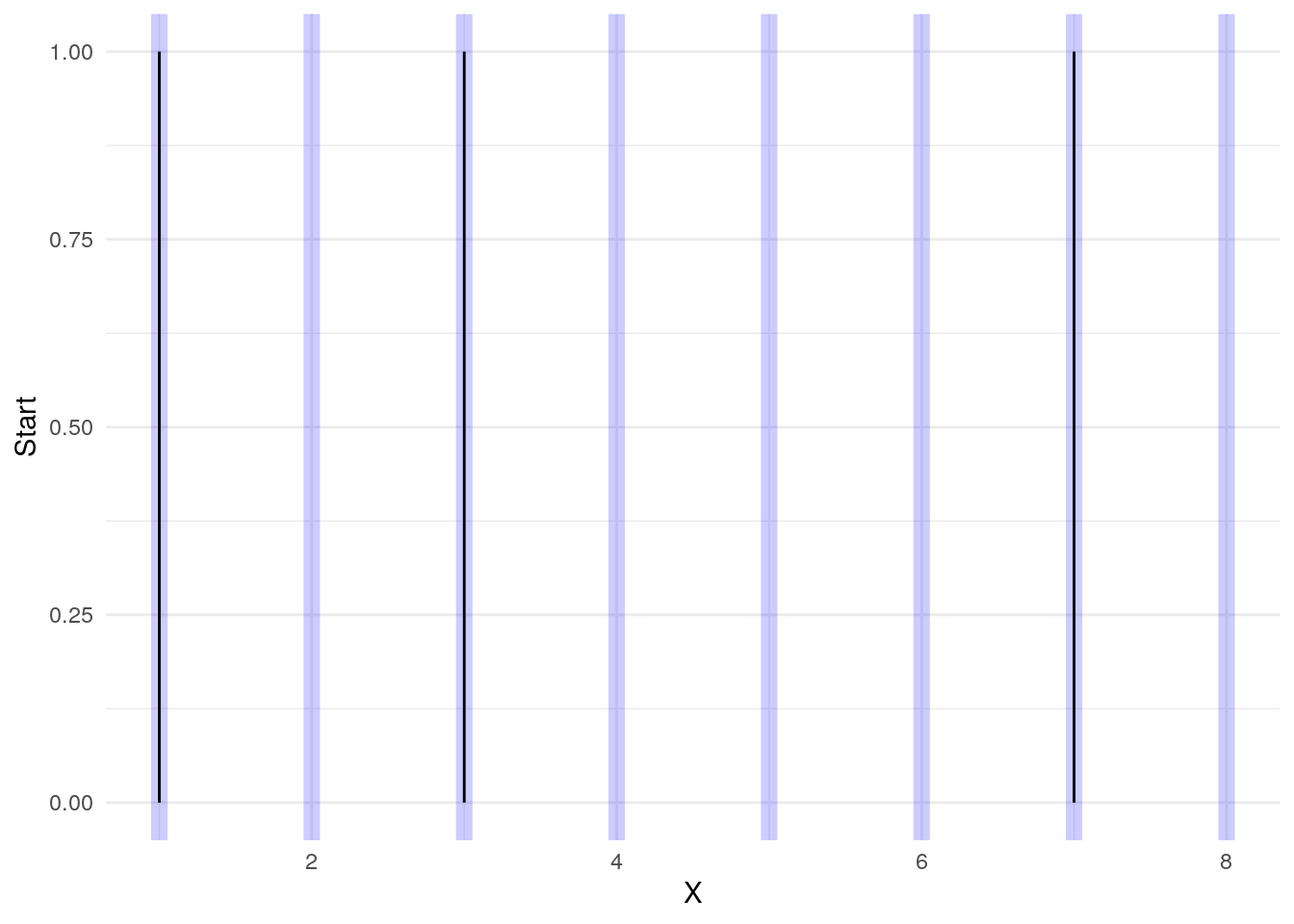
But we would like to group the records together:
| X | Start |
|---|---|
| 1 | 1 |
| 2 | 0 |
| 3 | 1 |
| 4 | 0 |
| 5 | 0 |
| 6 | 0 |
| 7 | 1 |
| 8 | 0 |
The trick to marking these records as belonging together is to use cumsum on the Start events
dta1$G <- cumsum( dta1$Start )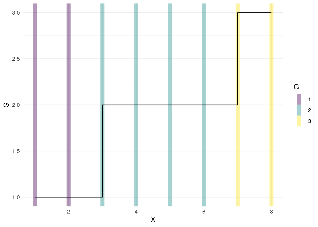
| X | Start | G |
|---|---|---|
| 1 | 1 | 1 |
| 2 | 0 | 1 |
| 3 | 1 | 2 |
| 4 | 0 | 2 |
| 5 | 0 | 2 |
| 6 | 0 | 2 |
| 7 | 1 | 3 |
| 8 | 0 | 3 |
The G column can be used in grouped calculations to identify each group of records.
Note that diff and cumsum are useful in this way when the data records are in increasing “time” order. It may be necessary to sort your data before applying these tools to it.
Intervals
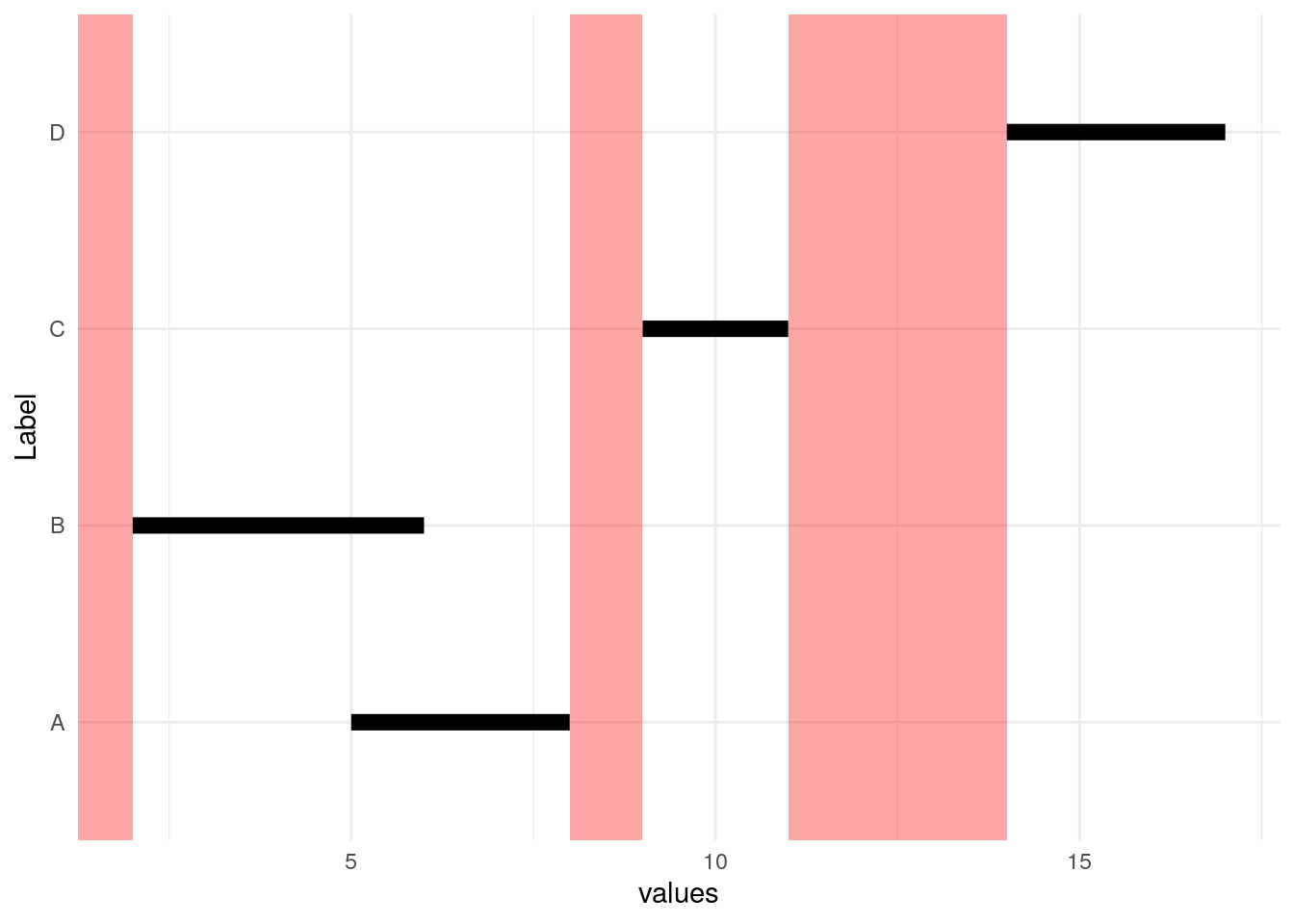
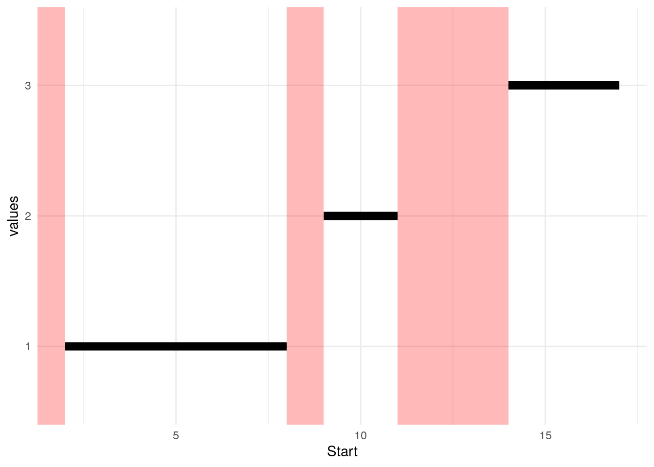
Now we look at a more involved extension of this idea: collapsing records that redundantly specify overlapping intervals.
dta2 <- read.table( text=
"Label Start End
A      5     8
B      2     6
C      9     11
D      14    17
",header=TRUE)| Label | Start | End |
|---|---|---|
| A | 5 | 8 |
| B | 2 | 6 |
| C | 9 | 11 |
| D | 14 | 17 |
As we see below, there are parts of the number line that are not identified by these Start/End pairs (red bars), and there are individual intervals shown by the black bars. Intervals A and B overlap, so the goal is to represent them by one black bar.
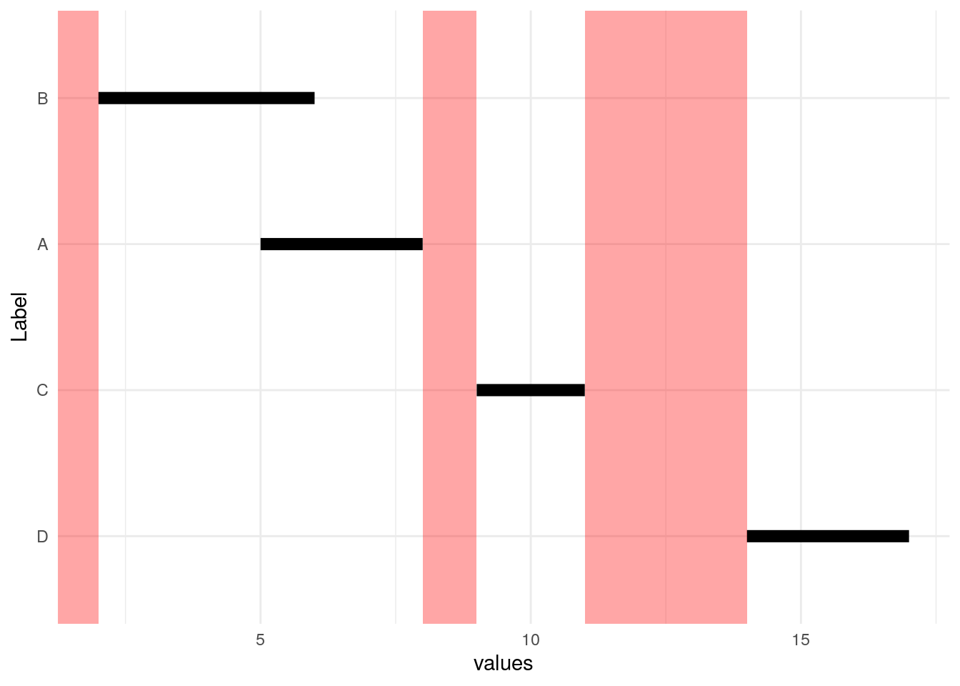
We start by sorting by beginning of interval (Start).
| Label | Start | End |
|---|---|---|
| B | 2 | 6 |
| A | 5 | 8 |
| C | 9 | 11 |
| D | 14 | 17 |
Next we notice that we can subtract the red End values from the yellow Start values to figure out how big the “hole” is preceding each Start value. Notice that the hole before the first interval is infinitely large.
| Label | Start | End |
|---|---|---|
| B | 2 | 6 |
| A | 5 | 8 |
| C | 9 | 11 |
| D | 14 | 17 |
dta2c <- (   dta2b
         %>% mutate( hole = c( Inf, Start[-1]-End[-n()] ) )
)| Label | Start | End | hole |
|---|---|---|---|
| B | 2 | 6 | Inf |
| A | 5 | 8 | -1 |
| C | 9 | 11 | 1 |
| D | 14 | 17 | 3 |
Next we identify events… which intervals have holes greater or equal to zero in front of them?
dta2d <- (   dta2c
         %>% mutate( group_start = ( 0 <= hole ) )
)| Label | Start | End | hole | group_start |
|---|---|---|---|---|
| B | 2 | 6 | Inf | TRUE |
| A | 5 | 8 | -1 | FALSE |
| C | 9 | 11 | 1 | TRUE |
| D | 14 | 17 | 3 | TRUE |
Now that we have events identified, we can use cumsum to identify records that belong together:
dta2e <- (   dta2d
         %>% mutate( group = cumsum( group_start ) )
)| Label | Start | End | hole | group_start | group |
|---|---|---|---|---|---|
| B | 2 | 6 | Inf | TRUE | 1 |
| A | 5 | 8 | -1 | FALSE | 1 |
| C | 9 | 11 | 1 | TRUE | 2 |
| D | 14 | 17 | 3 | TRUE | 3 |
With the group column defined, the minimum Start and the maximum End in each group value can be used to form a single interval record.
dta2f <- (   dta2e
         %>% group_by( group )
         %>% summarise( Start = min( Start )
                      , End = max( End )
                      )
         %>% ungroup()
)| group | Start | End |
|---|---|---|
| 1 | 2 | 8 |
| 2 | 9 | 11 |
| 3 | 14 | 17 |
With dplyr this series of operations can be piped together instead of built incrementally as we did above to show the intermediate results:
dta2g <- (   dta2
         %>% arrange( Start )
         %>% mutate( hole = c( Inf, Start[-1]-End[-n()] )
                   , group = cumsum( 0 <= hole )
                   )
         %>% group_by( group )
         %>% summarise( Start = min( Start )
                      , End = max( End )
                      )
         %>% ungroup()
)| group | Start | End |
|---|---|---|
| 1 | 2 | 8 |
| 2 | 9 | 11 |
| 3 | 14 | 17 |
One day (max) separation
Suppose you have intervals that are always defined using dates within one year, so technically December 31 does not actually overlap with January 1 of the following year. Depending on the nature of the data this may in fact be close enough, so you may want to define “overlap” as “within one day”. Consider a sample data set:
library(dplyr)

dta3 <- read.csv(text=
"id|start|end
1|2015-08-01|2015-12-31
1|2016-01-01|2016-12-31
1|2017-01-01|2017-05-08
2|2014-08-12|2014-12-31
2|2015-01-01|2015-07-23
2|2016-01-12|2016-12-31
2|2017-01-01|2017-08-22
",sep="|",as.is=TRUE
,colClasses=c("numeric","Date","Date"))
We can again compute hole size, and compare the hole size with 1 day instead of 0 days:
dta3a <- (   dta3
         %>% arrange( id, start )
         %>% group_by( id )
         %>% mutate( hole = c( Inf
                             , as.numeric( start[-1]-end[-n()]
                                         , units="days"
                                         )
                             )
                   , gp = cumsum( 1 < hole )
                   )
         %>% ungroup()
)| id | start | end | hole | gp |
|---|---|---|---|---|
| 1 | 2015-08-01 | 2015-12-31 | Inf | 1 |
| 1 | 2016-01-01 | 2016-12-31 | 1 | 1 |
| 1 | 2017-01-01 | 2017-05-08 | 1 | 1 |
| 2 | 2014-08-12 | 2014-12-31 | Inf | 1 |
| 2 | 2015-01-01 | 2015-07-23 | 1 | 1 |
| 2 | 2016-01-12 | 2016-12-31 | 173 | 2 |
| 2 | 2017-01-01 | 2017-08-22 | 1 | 2 |
Take this same sequence of calculations, and performing the group-by we can identify the starting date and the ending date for each group.
dta3b <- (   dta3
         %>% arrange( id, start )
         %>% group_by( id )
         %>% mutate( hole = c( Inf
                             , as.numeric( start[-1]-end[-n()]
                                         , units="days"
                                         )
                             )
                   , gp = cumsum( 1 < hole )
                   )
         %>% ungroup()
         %>% group_by( id, gp )
         %>% summarise( start = min( start )
                      , end = max( end )
                      )
)| id | gp | start | end |
|---|---|---|---|
| 1 | 1 | 2015-08-01 | 2017-05-08 |
| 2 | 1 | 2014-08-12 | 2015-07-23 |
| 2 | 2 | 2016-01-12 | 2017-08-22 |
Wind Direction
In a question on the R-help mailing list, the following problem is posed:
[…] the wind direction is very stable during these situations, and therefore I would like to start from it. […]
In the case of the example below reported, I know that the directions of this particular automatic station must be only SW or WSW.
My biggest problem, […] is to find the beginning and the end of each event, when there is a change in the main direction. Thinking about categorical data in general, is there a way to detect periods when one particular category is more frequent?
So the sample data provided is one day of wind data, with the intent to handle many days of data efficiently:
first_day_POSIX <- as.POSIXct( "2020-02-19" )
last_day_POSIX <- as.POSIXct( "2020-02-20" )
mydf <- data.frame(
    data_POSIX = seq( first_day_POSIX, last_day_POSIX, by="10 min" )
  , main_dir = c( "WSW", "WSW", "SW", "SW", "W", "WSW", "WSW", "WSW", "W"
                , "W", "SW", "WSW", "SSW", "S", "SW", "SW", "WSW", "WNW"
                , "W", "WSW", "WSW", "SE", "SE", "SE", "NW", "NNE", "ENE"
                , "SE", "NNW", "NW", "NW", "NW", "NW", "NW", "NW", "NE"
                , "NW", "NW", "NW", "NW", "NW", "N", "WNW", "NW", "NNW"
                , "NNW", "NW", "NW", "NW", "WNW", "ESE", "W", "WSW", "SW"
                , "SW", "SW", "WSW", "SW", "S", "S", "SSW", "SW", "WSW"
                , "WSW", "WSW", "WSW", "WSW", "WSW", "WSW", "SW", "WSW"
                , "WSW", "WSW", "WSW", "SW", "SW", "WSW", "WSW", "WSW"
                , "WSW", "WSW", "SW", "SW", "SW", "SW", "SW", "SW", "SW"
                , "SW", "SW", "WSW", "WSW", "WSW", "WSW", "SW", "SW"
                , "SW", "SW", "WSW", "SW", "SW", "SW", "SW", "SW", "WSW"
                , "SW", "SW", "W", "WSW", "WSW", "SSW", "S", "WNW", "SW"
                , "W", "WSW", "WSW", "SE", "SE", "SE", "NW", "NNE", "ENE"
                , "SE", "NNW", "NW", "NW", "NW", "NW", "NW", "NW", "NE"
                , "NW", "NW", "NW", "NW", "NW", "N", "WNW", "NW", "NNW"
                , "NNW", "NW", "NW", "NW"
                )
  , max_speed = c( 4.60, 4.60, 3.40, 3.10, 4.80, 4.20, 4.10, 4.50, 4.70
                 , 4.30, 2.40, 2.30, 2.20, 2.10, 2.90, 2.80, 1.80, 2.70
                 , 4.30, 3.30, 2.30, 2.30, 3.20, 3.20, 2.90, 2.30, 1.50
                 , 1.80, 2.90, 2.40, 1.80, 2.40, 2.30, 2.60, 1.80, 2.30
                 , 1.90, 2.20, 2.80, 2.40, 1.00, 1.10, 1.60, 2.30, 2.50
                 , 3.30, 3.40, 3.20, 4.50, 3.90, 3.10, 2.40, 6.00, 7.80
                 , 6.30, 7.80, 8.10, 6.10, 7.40, 9.50, 8.90, 9.10, 10.10
                 , 10.50, 11.10, 10.10, 10.90, 11.30, 13.40, 13.50, 12.80
                 , 11.50, 13.10, 13.50, 11.10, 10.50, 8.50, 10.10, 10.70
                 , 13.60, 11.90, 14.90, 10.90, 10.90, 12.80, 12.10, 9.10
                 , 8.30, 8.80, 7.40, 8.40, 10.30, 10.00, 7.00, 8.50, 8.40
                 , 8.60, 6.70, 7.30, 6.20, 5.90, 5.90, 5.10, 5.80, 5.60
                 , 6.50, 6.60, 11.70, 11.30, 8.70, 7.10, 6.90, 4.30
                 , 3.80, 4.30, 3.30, 2.30, 2.30, 3.20, 3.20, 2.90, 2.30
                 , 1.50, 1.80, 2.90, 2.40, 1.80, 2.40, 2.30, 2.60, 1.80
                 , 2.30, 1.90, 2.20, 2.80, 2.40, 1.00, 1.10, 1.60, 2.30
                 , 2.50, 3.30, 3.40, 3.20, 4.50
                 )
)
We begin with the base-R approach. Afterward this we will show the equivalent dplyr syntax.
First To identify candidate records to be considered as “foehn” conditions, and a first stab at the groups of records of interest:
mydf$foehn1a <- mydf$main_dir %in% c( "WSW", "SW" )
mydf$foehn1b <- cumsum( !mydf$foehn1a )
Having the ability to consider the groups separately, we identify sequences of records of more than ten records (one hour, as an example minimum period of time):
mydf$foehn1c <- ave( rep( 1, nrow( mydf ) )
                   , mydf$foehn1b
                   , FUN=function(v) 10 < length( v )
                   )
(If you are not familiar with the ave function, it calls the given function with subsets from the first argument corresponding to distinct values in the second argument (the grouping variable), and combines the results as a vector just as long as the original input data. The function should return either a scalar (which will be extended as necessary), or a vector the same length as the input vector.)
With the groups of similar-direction records that are long enough, we can re-compute events that only apply to the beginning of long intervals:
mydf$foehn1d <- 0 < diff( c( 0, mydf$foehn1c ) )Now we can generate distinct incrementing groups of records, and use the previously determined flag values for the long records to zero out the grouping flags for records that do not apply to the relevant “foehn” period of time:
mydf$foehn1e <- with( mydf
                    , ifelse( foehn1c
                            , cumsum( foehn1d )
                            , 0
                            )
)| data_POSIX | main_dir | max_speed | foehn1a | foehn1b | foehn1c | foehn1d | foehn1e |
|---|---|---|---|---|---|---|---|
| 2020-02-19 00:00:00 | WSW | 4.6 | TRUE | 0 | 0 | FALSE | 0 |
| 2020-02-19 00:10:00 | WSW | 4.6 | TRUE | 0 | 0 | FALSE | 0 |
| 2020-02-19 00:20:00 | SW | 3.4 | TRUE | 0 | 0 | FALSE | 0 |
| 2020-02-19 00:30:00 | SW | 3.1 | TRUE | 0 | 0 | FALSE | 0 |
| 2020-02-19 00:40:00 | W | 4.8 | FALSE | 1 | 0 | FALSE | 0 |
| 2020-02-19 00:50:00 | WSW | 4.2 | TRUE | 1 | 0 | FALSE | 0 |
| 2020-02-19 01:00:00 | WSW | 4.1 | TRUE | 1 | 0 | FALSE | 0 |
| 2020-02-19 01:10:00 | WSW | 4.5 | TRUE | 1 | 0 | FALSE | 0 |
| 2020-02-19 01:20:00 | W | 4.7 | FALSE | 2 | 0 | FALSE | 0 |
| 2020-02-19 01:30:00 | W | 4.3 | FALSE | 3 | 0 | FALSE | 0 |
| 2020-02-19 01:40:00 | SW | 2.4 | TRUE | 3 | 0 | FALSE | 0 |
| 2020-02-19 01:50:00 | WSW | 2.3 | TRUE | 3 | 0 | FALSE | 0 |
| 2020-02-19 02:00:00 | SSW | 2.2 | FALSE | 4 | 0 | FALSE | 0 |
| 2020-02-19 02:10:00 | S | 2.1 | FALSE | 5 | 0 | FALSE | 0 |
| 2020-02-19 02:20:00 | SW | 2.9 | TRUE | 5 | 0 | FALSE | 0 |
| 2020-02-19 02:30:00 | SW | 2.8 | TRUE | 5 | 0 | FALSE | 0 |
| 2020-02-19 02:40:00 | WSW | 1.8 | TRUE | 5 | 0 | FALSE | 0 |
| 2020-02-19 02:50:00 | WNW | 2.7 | FALSE | 6 | 0 | FALSE | 0 |
| 2020-02-19 03:00:00 | W | 4.3 | FALSE | 7 | 0 | FALSE | 0 |
| 2020-02-19 03:10:00 | WSW | 3.3 | TRUE | 7 | 0 | FALSE | 0 |
| 2020-02-19 03:20:00 | WSW | 2.3 | TRUE | 7 | 0 | FALSE | 0 |
| 2020-02-19 03:30:00 | SE | 2.3 | FALSE | 8 | 0 | FALSE | 0 |
| 2020-02-19 03:40:00 | SE | 3.2 | FALSE | 9 | 0 | FALSE | 0 |
| 2020-02-19 03:50:00 | SE | 3.2 | FALSE | 10 | 0 | FALSE | 0 |
| 2020-02-19 04:00:00 | NW | 2.9 | FALSE | 11 | 0 | FALSE | 0 |
| 2020-02-19 04:10:00 | NNE | 2.3 | FALSE | 12 | 0 | FALSE | 0 |
| 2020-02-19 04:20:00 | ENE | 1.5 | FALSE | 13 | 0 | FALSE | 0 |
| 2020-02-19 04:30:00 | SE | 1.8 | FALSE | 14 | 0 | FALSE | 0 |
| 2020-02-19 04:40:00 | NNW | 2.9 | FALSE | 15 | 0 | FALSE | 0 |
| 2020-02-19 04:50:00 | NW | 2.4 | FALSE | 16 | 0 | FALSE | 0 |
| 2020-02-19 05:00:00 | NW | 1.8 | FALSE | 17 | 0 | FALSE | 0 |
| 2020-02-19 05:10:00 | NW | 2.4 | FALSE | 18 | 0 | FALSE | 0 |
| 2020-02-19 05:20:00 | NW | 2.3 | FALSE | 19 | 0 | FALSE | 0 |
| 2020-02-19 05:30:00 | NW | 2.6 | FALSE | 20 | 0 | FALSE | 0 |
| 2020-02-19 05:40:00 | NW | 1.8 | FALSE | 21 | 0 | FALSE | 0 |
| 2020-02-19 05:50:00 | NE | 2.3 | FALSE | 22 | 0 | FALSE | 0 |
| 2020-02-19 06:00:00 | NW | 1.9 | FALSE | 23 | 0 | FALSE | 0 |
| 2020-02-19 06:10:00 | NW | 2.2 | FALSE | 24 | 0 | FALSE | 0 |
| 2020-02-19 06:20:00 | NW | 2.8 | FALSE | 25 | 0 | FALSE | 0 |
| 2020-02-19 06:30:00 | NW | 2.4 | FALSE | 26 | 0 | FALSE | 0 |
| 2020-02-19 06:40:00 | NW | 1.0 | FALSE | 27 | 0 | FALSE | 0 |
| 2020-02-19 06:50:00 | N | 1.1 | FALSE | 28 | 0 | FALSE | 0 |
| 2020-02-19 07:00:00 | WNW | 1.6 | FALSE | 29 | 0 | FALSE | 0 |
| 2020-02-19 07:10:00 | NW | 2.3 | FALSE | 30 | 0 | FALSE | 0 |
| 2020-02-19 07:20:00 | NNW | 2.5 | FALSE | 31 | 0 | FALSE | 0 |
| 2020-02-19 07:30:00 | NNW | 3.3 | FALSE | 32 | 0 | FALSE | 0 |
| 2020-02-19 07:40:00 | NW | 3.4 | FALSE | 33 | 0 | FALSE | 0 |
| 2020-02-19 07:50:00 | NW | 3.2 | FALSE | 34 | 0 | FALSE | 0 |
| 2020-02-19 08:00:00 | NW | 4.5 | FALSE | 35 | 0 | FALSE | 0 |
| 2020-02-19 08:10:00 | WNW | 3.9 | FALSE | 36 | 0 | FALSE | 0 |
| 2020-02-19 08:20:00 | ESE | 3.1 | FALSE | 37 | 0 | FALSE | 0 |
| 2020-02-19 08:30:00 | W | 2.4 | FALSE | 38 | 0 | FALSE | 0 |
| 2020-02-19 08:40:00 | WSW | 6.0 | TRUE | 38 | 0 | FALSE | 0 |
| 2020-02-19 08:50:00 | SW | 7.8 | TRUE | 38 | 0 | FALSE | 0 |
| 2020-02-19 09:00:00 | SW | 6.3 | TRUE | 38 | 0 | FALSE | 0 |
| 2020-02-19 09:10:00 | SW | 7.8 | TRUE | 38 | 0 | FALSE | 0 |
| 2020-02-19 09:20:00 | WSW | 8.1 | TRUE | 38 | 0 | FALSE | 0 |
| 2020-02-19 09:30:00 | SW | 6.1 | TRUE | 38 | 0 | FALSE | 0 |
| 2020-02-19 09:40:00 | S | 7.4 | FALSE | 39 | 0 | FALSE | 0 |
| 2020-02-19 09:50:00 | S | 9.5 | FALSE | 40 | 0 | FALSE | 0 |
| 2020-02-19 10:00:00 | SSW | 8.9 | FALSE | 41 | 1 | TRUE | 1 |
| 2020-02-19 10:10:00 | SW | 9.1 | TRUE | 41 | 1 | FALSE | 1 |
| 2020-02-19 10:20:00 | WSW | 10.1 | TRUE | 41 | 1 | FALSE | 1 |
| 2020-02-19 10:30:00 | WSW | 10.5 | TRUE | 41 | 1 | FALSE | 1 |
| 2020-02-19 10:40:00 | WSW | 11.1 | TRUE | 41 | 1 | FALSE | 1 |
| 2020-02-19 10:50:00 | WSW | 10.1 | TRUE | 41 | 1 | FALSE | 1 |
| 2020-02-19 11:00:00 | WSW | 10.9 | TRUE | 41 | 1 | FALSE | 1 |
| 2020-02-19 11:10:00 | WSW | 11.3 | TRUE | 41 | 1 | FALSE | 1 |
| 2020-02-19 11:20:00 | WSW | 13.4 | TRUE | 41 | 1 | FALSE | 1 |
| 2020-02-19 11:30:00 | SW | 13.5 | TRUE | 41 | 1 | FALSE | 1 |
| 2020-02-19 11:40:00 | WSW | 12.8 | TRUE | 41 | 1 | FALSE | 1 |
| 2020-02-19 11:50:00 | WSW | 11.5 | TRUE | 41 | 1 | FALSE | 1 |
| 2020-02-19 12:00:00 | WSW | 13.1 | TRUE | 41 | 1 | FALSE | 1 |
| 2020-02-19 12:10:00 | WSW | 13.5 | TRUE | 41 | 1 | FALSE | 1 |
| 2020-02-19 12:20:00 | SW | 11.1 | TRUE | 41 | 1 | FALSE | 1 |
| 2020-02-19 12:30:00 | SW | 10.5 | TRUE | 41 | 1 | FALSE | 1 |
| 2020-02-19 12:40:00 | WSW | 8.5 | TRUE | 41 | 1 | FALSE | 1 |
| 2020-02-19 12:50:00 | WSW | 10.1 | TRUE | 41 | 1 | FALSE | 1 |
| 2020-02-19 13:00:00 | WSW | 10.7 | TRUE | 41 | 1 | FALSE | 1 |
| 2020-02-19 13:10:00 | WSW | 13.6 | TRUE | 41 | 1 | FALSE | 1 |
| 2020-02-19 13:20:00 | WSW | 11.9 | TRUE | 41 | 1 | FALSE | 1 |
| 2020-02-19 13:30:00 | SW | 14.9 | TRUE | 41 | 1 | FALSE | 1 |
| 2020-02-19 13:40:00 | SW | 10.9 | TRUE | 41 | 1 | FALSE | 1 |
| 2020-02-19 13:50:00 | SW | 10.9 | TRUE | 41 | 1 | FALSE | 1 |
| 2020-02-19 14:00:00 | SW | 12.8 | TRUE | 41 | 1 | FALSE | 1 |
| 2020-02-19 14:10:00 | SW | 12.1 | TRUE | 41 | 1 | FALSE | 1 |
| 2020-02-19 14:20:00 | SW | 9.1 | TRUE | 41 | 1 | FALSE | 1 |
| 2020-02-19 14:30:00 | SW | 8.3 | TRUE | 41 | 1 | FALSE | 1 |
| 2020-02-19 14:40:00 | SW | 8.8 | TRUE | 41 | 1 | FALSE | 1 |
| 2020-02-19 14:50:00 | SW | 7.4 | TRUE | 41 | 1 | FALSE | 1 |
| 2020-02-19 15:00:00 | WSW | 8.4 | TRUE | 41 | 1 | FALSE | 1 |
| 2020-02-19 15:10:00 | WSW | 10.3 | TRUE | 41 | 1 | FALSE | 1 |
| 2020-02-19 15:20:00 | WSW | 10.0 | TRUE | 41 | 1 | FALSE | 1 |
| 2020-02-19 15:30:00 | WSW | 7.0 | TRUE | 41 | 1 | FALSE | 1 |
| 2020-02-19 15:40:00 | SW | 8.5 | TRUE | 41 | 1 | FALSE | 1 |
| 2020-02-19 15:50:00 | SW | 8.4 | TRUE | 41 | 1 | FALSE | 1 |
| 2020-02-19 16:00:00 | SW | 8.6 | TRUE | 41 | 1 | FALSE | 1 |
| 2020-02-19 16:10:00 | SW | 6.7 | TRUE | 41 | 1 | FALSE | 1 |
| 2020-02-19 16:20:00 | WSW | 7.3 | TRUE | 41 | 1 | FALSE | 1 |
| 2020-02-19 16:30:00 | SW | 6.2 | TRUE | 41 | 1 | FALSE | 1 |
| 2020-02-19 16:40:00 | SW | 5.9 | TRUE | 41 | 1 | FALSE | 1 |
| 2020-02-19 16:50:00 | SW | 5.9 | TRUE | 41 | 1 | FALSE | 1 |
| 2020-02-19 17:00:00 | SW | 5.1 | TRUE | 41 | 1 | FALSE | 1 |
| 2020-02-19 17:10:00 | SW | 5.8 | TRUE | 41 | 1 | FALSE | 1 |
| 2020-02-19 17:20:00 | WSW | 5.6 | TRUE | 41 | 1 | FALSE | 1 |
| 2020-02-19 17:30:00 | SW | 6.5 | TRUE | 41 | 1 | FALSE | 1 |
| 2020-02-19 17:40:00 | SW | 6.6 | TRUE | 41 | 1 | FALSE | 1 |
| 2020-02-19 17:50:00 | W | 11.7 | FALSE | 42 | 0 | FALSE | 0 |
| 2020-02-19 18:00:00 | WSW | 11.3 | TRUE | 42 | 0 | FALSE | 0 |
| 2020-02-19 18:10:00 | WSW | 8.7 | TRUE | 42 | 0 | FALSE | 0 |
| 2020-02-19 18:20:00 | SSW | 7.1 | FALSE | 43 | 0 | FALSE | 0 |
| 2020-02-19 18:30:00 | S | 6.9 | FALSE | 44 | 0 | FALSE | 0 |
| 2020-02-19 18:40:00 | WNW | 4.3 | FALSE | 45 | 0 | FALSE | 0 |
| 2020-02-19 18:50:00 | SW | 3.8 | TRUE | 45 | 0 | FALSE | 0 |
| 2020-02-19 19:00:00 | W | 4.3 | FALSE | 46 | 0 | FALSE | 0 |
| 2020-02-19 19:10:00 | WSW | 3.3 | TRUE | 46 | 0 | FALSE | 0 |
| 2020-02-19 19:20:00 | WSW | 2.3 | TRUE | 46 | 0 | FALSE | 0 |
| 2020-02-19 19:30:00 | SE | 2.3 | FALSE | 47 | 0 | FALSE | 0 |
| 2020-02-19 19:40:00 | SE | 3.2 | FALSE | 48 | 0 | FALSE | 0 |
| 2020-02-19 19:50:00 | SE | 3.2 | FALSE | 49 | 0 | FALSE | 0 |
| 2020-02-19 20:00:00 | NW | 2.9 | FALSE | 50 | 0 | FALSE | 0 |
| 2020-02-19 20:10:00 | NNE | 2.3 | FALSE | 51 | 0 | FALSE | 0 |
| 2020-02-19 20:20:00 | ENE | 1.5 | FALSE | 52 | 0 | FALSE | 0 |
| 2020-02-19 20:30:00 | SE | 1.8 | FALSE | 53 | 0 | FALSE | 0 |
| 2020-02-19 20:40:00 | NNW | 2.9 | FALSE | 54 | 0 | FALSE | 0 |
| 2020-02-19 20:50:00 | NW | 2.4 | FALSE | 55 | 0 | FALSE | 0 |
| 2020-02-19 21:00:00 | NW | 1.8 | FALSE | 56 | 0 | FALSE | 0 |
| 2020-02-19 21:10:00 | NW | 2.4 | FALSE | 57 | 0 | FALSE | 0 |
| 2020-02-19 21:20:00 | NW | 2.3 | FALSE | 58 | 0 | FALSE | 0 |
| 2020-02-19 21:30:00 | NW | 2.6 | FALSE | 59 | 0 | FALSE | 0 |
| 2020-02-19 21:40:00 | NW | 1.8 | FALSE | 60 | 0 | FALSE | 0 |
| 2020-02-19 21:50:00 | NE | 2.3 | FALSE | 61 | 0 | FALSE | 0 |
| 2020-02-19 22:00:00 | NW | 1.9 | FALSE | 62 | 0 | FALSE | 0 |
| 2020-02-19 22:10:00 | NW | 2.2 | FALSE | 63 | 0 | FALSE | 0 |
| 2020-02-19 22:20:00 | NW | 2.8 | FALSE | 64 | 0 | FALSE | 0 |
| 2020-02-19 22:30:00 | NW | 2.4 | FALSE | 65 | 0 | FALSE | 0 |
| 2020-02-19 22:40:00 | NW | 1.0 | FALSE | 66 | 0 | FALSE | 0 |
| 2020-02-19 22:50:00 | N | 1.1 | FALSE | 67 | 0 | FALSE | 0 |
| 2020-02-19 23:00:00 | WNW | 1.6 | FALSE | 68 | 0 | FALSE | 0 |
| 2020-02-19 23:10:00 | NW | 2.3 | FALSE | 69 | 0 | FALSE | 0 |
| 2020-02-19 23:20:00 | NNW | 2.5 | FALSE | 70 | 0 | FALSE | 0 |
| 2020-02-19 23:30:00 | NNW | 3.3 | FALSE | 71 | 0 | FALSE | 0 |
| 2020-02-19 23:40:00 | NW | 3.4 | FALSE | 72 | 0 | FALSE | 0 |
| 2020-02-19 23:50:00 | NW | 3.2 | FALSE | 73 | 0 | FALSE | 0 |
| 2020-02-20 00:00:00 | NW | 4.5 | FALSE | 74 | 0 | FALSE | 0 |
And if all we want is to identify start and end periods:
mydf1 <- mydf[ 0 != mydf$foehn1e, c( "data_POSIX", "foehn1e") ]
mydf2 <- do.call( rbind
                , lapply( split( mydf1
                               , mydf1$foehn1e
                               )
                        , function( DF ) {
                            data.frame( foehn1e = DF$foehn1e[ 1 ]
                                      , Start = min( DF$data_POSIX )
                                      , End = max( DF$data_POSIX )
                                      )
                          }
                        )
)| foehn1e | Start | End |
|---|---|---|
| 1 | 2020-02-19 10:00:00 | 2020-02-19 17:40:00 |
Alternatively, the above steps can be encoded using dplyr:
mydf3alt <- (   mydf
            %>% mutate( foehn1a = main_dir %in% c( "WSW", "SW" )
                      , foehn1b = cumsum( !foehn1a )
                      )
            %>% group_by( foehn1b )
            %>% mutate( foehn1c = 10 < n() )
            %>% ungroup()
            %>% mutate( foehn1d = 0 < diff( c( 0, foehn1c ) )
                      , foehn1e = ifelse( foehn1c
                                        , cumsum( foehn1d )
                                        , 0
                                        )
                      )
            )
Just to confirm that this method obtains the same result as the base R method:
all( mydf == mydf3alt )## [1] TRUEAnd the collapsed form is:
mydf3alt2 <- (   mydf3alt
             %>% filter( 0 < foehn1e )
             %>% group_by( foehn1e )
             %>% summarise( Start = min( data_POSIX )
                          , End = max( data_POSIX )
                          )
)| foehn1e | Start | End |
|---|---|---|
| 1 | 2020-02-19 10:00:00 | 2020-02-19 17:40:00 |
Just to confirm the same final results:
all( mydf2 == mydf3alt2 )## [1] TRUE👍
Fini
In summary:
- The
difffunction is useful in finding “events” to begin or end groups of record classifications. - Events can also be identified using logical tests of information in records.
- The
cumsumfunction is useful in converting events into grouping variables. - These grouping columns can be used to divide up the records into groups and collapse them into summary values such as start or end times, or aggregate measures relevant to those records.
- These techniques can efficiently scale up to very large data sets.
- There are some forms of event specifications that cannot be identified this way, and in such cases a for loop in R or Rcpp may be needed. In general, when continuous values are accumulated differently according to events, and subsequent events are defined in terms of those continuous accumulations, those simulations are in general not amenable to these
cumsumanddifftricks.