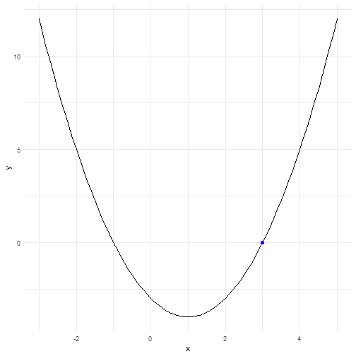
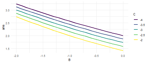
class: center, middle, inverse, title-slide # Do It Again, R! ## Intro to Loops, Functions and Groups ### Jeff Newmiller ### 7 May 2019 --- # Outline - For Loops + Where is my output? + Keeping results - Vectors of inputs and vectors of outputs¹ + Vectorized functions, not "Vectorize my function" + Appending columns + Plotting results: ggplot2 - Expanding options + Cartesian join: expand.grid .footnote[ [1] Inspired by _R for Data Science_ (https://r4ds.had.co.nz) ] --- # Packages Used ```r library(dplyr) # tidyverse library(ggplot2) # tidyverse library(purrr) # tidyverse library(microbenchmark) # speed check library(tidyr) # tidyverse ``` --- ## Sample Problem Given a relationship between `\(x\)` and `\(y\)`: $$ y = a x^2 + b x + c $$ we can find which values of `\(x\)` cause `\(y=0\)` using the quadratic formula: $$ x = \frac{-b \pm \sqrt{b^2-4ac}}{2a} $$ --- # Sample Solution For now, we will focus on the most positive answer: ```r A <- 1 ; B <- -2 ; C <- -3 DF1 <- tibble( x = seq( -3, 5, 0.1 ) , y = A*x^2 + B*x + C ) head( DF1, 4 ) ``` ``` ## # A tibble: 4 x 2 ## x y ## <dbl> <dbl> ## 1 -3 12 ## 2 -2.9 11.2 ## 3 -2.8 10.4 ## 4 -2.7 9.69 ``` ```r ans <- ( -B + sqrt( B^2 - 4*A*C ) ) / ( 2 * A ) DF1b <- tibble( x = ans, y = 0 ) ans ``` ``` ## [1] 3 ``` --- # Solution Plot <!-- --> --- # Do it more than once? ```r input <- read.csv( "data/MyABC1.csv" ) input ``` ``` ## Trial A B C ## 1 1 1 -2 -3 ## 2 2 1 -3 -4 ## 3 3 1 -4 -5 ``` --- # For Loop - Printing A common approach used in other languages is to print results as you go along: ```r for ( i in seq_along( input$A ) ) { A <- input$A[ i ] B <- input$B[ i ] C <- input$C[ i ] print( sprintf( "A = %8.4f, B = %8.4f, C = %8.4f, x = %8.4f" , A, B, C , ( -B + sqrt( B^2 - 4*A*C ) ) / ( 2 * A ) ) ) } ``` ``` ## [1] "A = 1.0000, B = -2.0000, C = -3.0000, x = 3.0000" ## [1] "A = 1.0000, B = -3.0000, C = -4.0000, x = 4.0000" ## [1] "A = 1.0000, B = -4.0000, C = -5.0000, x = 5.0000" ``` --- # For Loop - Concatenating Another common recommendation is to concatenate: ```r ans <- numeric( 0 ) for ( i in seq_along( input$A ) ) { A <- input$A[ i ] B <- input$B[ i ] C <- input$C[ i ] ans <- c( ans, ( -B + sqrt( B^2 - 4*A*C ) ) / ( 2 * A ) ) } ans ``` ``` ## [1] 3 4 5 ``` Concatenating can be _very_ inefficient if there are many elements of `ans` because there are `\(n-1\)` shorter versions of `ans` created and discarded along the way. --- # For Loop - Element Replacement Allocating a vector large enough to hold all the answers and then replacing one element at a time is noticeably faster. ```r ans <- numeric( nrow( input ) ) ans ``` ``` ## [1] 0 0 0 ``` ```r for ( i in seq_along( input$A ) ) { A <- input$A[ i ] ; B <- input$B[ i ] ; C <- input$C[ i ] ans[ i ] <- ( -B + sqrt( B^2 - 4*A*C ) ) / ( 2 * A ) } ans ``` ``` ## [1] 3 4 5 ``` --- # Combined Presentation Having your results in a vector of their own is useful, but showing that vector next to the inputs is even more useful: ```r cbind( input, tibble( ans = ans ) ) ``` ``` ## Trial A B C ans ## 1 1 1 -2 -3 3 ## 2 2 1 -3 -4 4 ## 3 3 1 -4 -5 5 ``` --- # Make a Solution Function To make a function, write code that uses inputs mentioned in the parentheses, and the last expression in the function will be the answer given by the function: ```r my_solution <- function( A, B, C ) { ( -B + sqrt( B^2 - 4*A*C ) ) / ( 2 * A ) } my_solution( 1, -2, -3 ) # try it out ``` ``` ## [1] 3 ``` You can also draw on variables from the working environment where you define the function, but it is intentionally hard to make changes to such variables inside a function. --- # Make a Many Solutions Function If your solutions generally only worked for one value each for `A`, `B`, and `C` then you might make this function: ```r my_many_solutions <- function( A, B, C, solution ) { ans <- numeric( length( A ) ) for ( i in seq_along( A ) ) { ans[ i ] <- solution( A[ i ], B[ i ], C[ i ] ) } ans } my_many_solutions( input$A, input$B, input$C, my_solution ) ``` ``` ## [1] 3 4 5 ``` --- # But why Re-Invent the Wheel? The `pmap_dbl` function takes a data frame and applies a function to each row. The function arguments have to be the same as the column names in the data frame, so we exclude the `Trial` column before giving it to `pmap_dbl`: ```r library(purrr) pmap_dbl( input[ , -1 ], my_solution ) ``` ``` ## [1] 3 4 5 ``` --- # Vectorized Calculations In this case, because R arithmetic operations are internally vectorized, the `my_solution` function can directly be given vectors instead of one value at a time, which is much faster: ```r my_solution( input$A, input$B, input$C ) ``` ``` ## [1] 3 4 5 ``` --- # Why Not Always Vectorize? Some algorithms are hard to implement in vectorized fashion... you may reach your goal sooner if you use a slower but simpler algorithm that is imperfect but gets the job done: ```r my_slow_solution <- function( A, B, C ) { Y <- function( X, A, B, C ) { A * X^2 + B * X + C } # only one answer at a time uniroot( Y, c( 0, 1e6 ), A = A, B = B, C = C, tol = 1e-8 )$root } my_slow_solution( 1, -2, -3 ) ``` ``` ## [1] 3 ``` but if you plan to solve many thousands or millions of problems, it may pay off to spend time making a complex algorithm vectorized. --- # Speed Review The price of flexibility when using `pmap_dbl` is speed. ```r options( digits = 1 ) # compact results library(microbenchmark) ans <- microbenchmark( loop_slow = my_many_solutions( input$A, input$B, input$C , my_slow_solution ) , pmap_slow = pmap_dbl( input[ , -1 ], my_slow_solution ) , loop_single = my_many_solutions( input$A, input$B, input$C , my_solution ) , pmap_single = pmap_dbl( input[ , -1 ], my_solution ) , vectorized = my_solution( input$A, input$B, input$C ) ) summary( ans ) ``` ``` ## expr min lq mean median uq max neval ## 1 loop_slow 221 231 398 294 463 4322 100 ## 2 pmap_slow 255 263 401 283 421 3486 100 ## 3 loop_single 17 21 30 24 35 77 100 ## 4 pmap_single 42 52 90 71 113 570 100 ## 5 vectorized 14 17 26 22 32 86 100 ``` --- # Expanding Options What if you want to try out a bunch of possible input combinations without listing all of them in a file? `expand.grid` to the rescue! ```r options( digits = 3 ) Bvals <- seq( -2, 0, 0.1 ) # 21 values Cvals <- seq( -4, -2, 0.5 ) # 5 values DF2 <- expand.grid( A = 1 # all combinations A/B/C , B = Bvals , C = Cvals ) nrow( DF2 ) # 1 * 5 * 21 ``` ``` ## [1] 105 ``` ```r head( DF2 ) ``` ``` ## A B C ## 1 1 -2.0 -4 ## 2 1 -1.9 -4 ## 3 1 -1.8 -4 ## 4 1 -1.7 -4 ## 5 1 -1.6 -4 ## 6 1 -1.5 -4 ``` --- # Computing on Combinations With so many ways to compute a vector of answers given an input data frame, we can choose the one most appropriate: ```r DF2$ans <- my_solution( DF2$A, DF2$B, DF2$C ) # 105 answers at once! head( DF2 ) ``` ``` ## A B C ans ## 1 1 -2.0 -4 3.24 ## 2 1 -1.9 -4 3.16 ## 3 1 -1.8 -4 3.09 ## 4 1 -1.7 -4 3.02 ## 5 1 -1.6 -4 2.95 ## 6 1 -1.5 -4 2.89 ``` Each row now has an answer associated with it. How should we present these results? --- # Grouping Rows One way is to treat each separate value of `C` distinctly, but plot `ans` vs. `B`. The usual way to mark a group of rows is to give them all the same value of a factor: ```r DF2$Cgroup <- factor( DF2$C # there are 105 elements... , levels = Cvals # but only 5 discrete values ) head( DF2 ) ``` ``` ## A B C ans Cgroup ## 1 1 -2.0 -4 3.24 -4 ## 2 1 -1.9 -4 3.16 -4 ## 3 1 -1.8 -4 3.09 -4 ## 4 1 -1.7 -4 3.02 -4 ## 5 1 -1.6 -4 2.95 -4 ## 6 1 -1.5 -4 2.89 -4 ``` --- # Use `ggplot2` Color Ggplot will separate the data into groups of records where the `Cgroup` column values are all the same. Note that because `C` is numeric, `ggplot` would assume if we used `C` for color there could be values like 3.7 even though we purposely skipped over that value. ```r library(ggplot2) ggplot( DF2, aes( x = B, y = ans, colour = Cgroup ) ) + geom_line( size = 1 ) + scale_color_viridis_d( name = "C" ) + theme_minimal() ``` <!-- --> --- # Output Sometimes others don't want a "long"-form data frame... the `spread` function is useful for "pivoting" your calculations to a more human-digestible layout: ```r library(tidyr) options( digits = 3 ) DF3 <- ( DF2 %>% select( A, B, Cgroup, ans ) %>% spread( Cgroup, ans ) ) head( DF3 ) ``` ``` ## A B -4 -3.5 -3 -2.5 -2 ## 1 1 -2.0 3.24 3.12 3.00 2.87 2.73 ## 2 1 -1.9 3.16 3.05 2.93 2.79 2.65 ## 3 1 -1.8 3.09 2.98 2.85 2.72 2.58 ## 4 1 -1.7 3.02 2.90 2.78 2.65 2.50 ## 5 1 -1.6 2.95 2.83 2.71 2.57 2.42 ## 6 1 -1.5 2.89 2.77 2.64 2.50 2.35 ``` The factor version of `C` is discrete, which makes it easier to know which `ans` values will end up in each column. --- # Conclusion - For loops are not always bad + Most useful for repeating `solution`s that involve a lot of calculations anyway + `apply`-type functions are just wrappers for `for` loops with results pre-allocation - Vectorized code uses all vector-based primitive operations + `apply`-type code _looks_ vectorized so easy to read, but not as fast + See `?Arithmetic`, and `?cumsum`, and `?rowSums` for example - Grouping rows by discrete values helps you sort out your results + Numeric values are not discrete, but you can fake it by making a factor - Do check out R4DS (https://r4ds.had.co.nz) for more useful analysis strategies .footnote[ [1] HTML slides built with the `xaringan` package, available via `install.packages`. ]