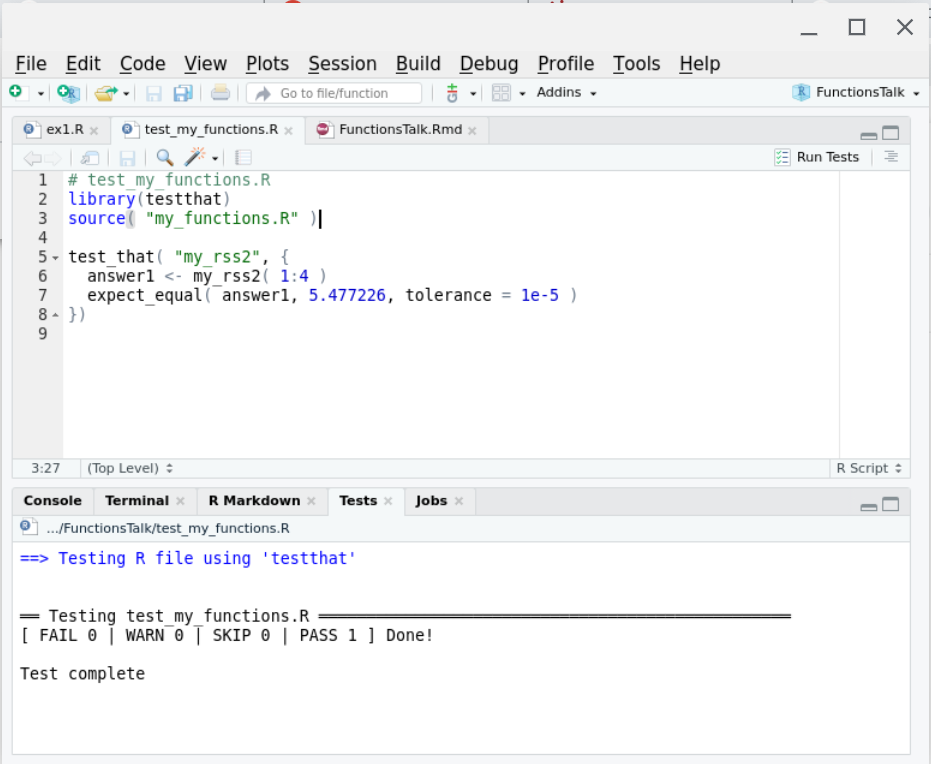
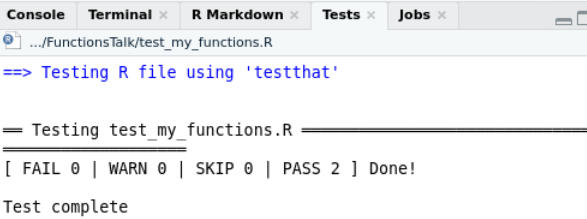
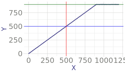
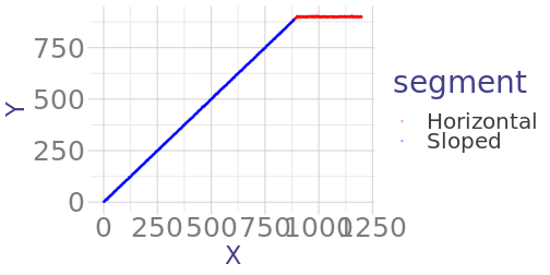
class: center, middle, inverse, title-slide # Some Notes on Functions ### Jeff Newmiller ### 9/14/2021 --- ## Outline - Common questions by beginners: + "I can't figure out how to make a function" + "I can't figure out what should be in the function" - In pursuit of answers + From script to function... + Three kinds of functions... + What's in a name... + Getting something working + Thinking in functions + Review --- class: title-slide, middle, inverse ## .center[From script to function...] --- ## What is a function? In R, functions are objects containing code that can be executed to do useful things. An example of a useful function in R is the `mean` function: ```r x <- 1:4 x ``` ``` ## [1] 1 2 3 4 ``` ```r result <- mean( x ) result ``` ``` ## [1] 2.5 ``` <div id="htmlwidget-bdc66eca06342b7a2f75" style="width:600px;height:100px;" class="grViz html-widget"></div> <script type="application/json" data-for="htmlwidget-bdc66eca06342b7a2f75">{"x":{"diagram":"digraph function {\nrankdir = LR\nnode [shape=none]\nx\nresult\nnode [shape=oval]\nx -> mean [label=\"[numeric vector]\"]\nmean -> result [label=\"[length 1 vector]\"]\n}\n","config":{"engine":"dot","options":null}},"evals":[],"jsHooks":[]}</script> --- ## Some code to re-use Suppose you have figured out how to compute the root-sum-square of some numbers, and now you want to be able to easily apply this algorithm to new data. This particular example is intentionally very small... we will look at more involved examples later. ```r y <- x^2 # x defined on previous slide as 1:4 y ``` ``` ## [1] 1 4 9 16 ``` ```r ysum <- sum( y ) ysum ``` ``` ## [1] 30 ``` ```r result <- sqrt( ysum ) result ``` ``` ## [1] 5.477226 ``` --- ## Wrap your code in a function definition ```r *my_rss1 <- function() { # first added line y <- x^2 # untouched code y # untouched code ysum <- sum( y ) # untouched code ysum # untouched code result <- sqrt( ysum ) # untouched code result # untouched code - value to return *} # second added line my_rss1() # test the new function my_rss1 ``` ``` ## [1] 5.477226 ``` This lets us type `my_rss1()` to do all the work of those "untouched code" lines in one short step. But one thing to notice about this is that we haven't defined any arguments yet... the code is using the `x` variable that we had defined in the global environment from earlier. This is a problem because remembering to create that variable before calling this function is hard. --- ## What if we forget? ```r rm( x ) # What if the x variable doesn't exist? my_rss1() # call function again, but don't have # global variable x defined ``` ``` Error in my_rss1() : object 'x' not found ``` We normally identify the outside variables we want (parameters) with internal names in the function (arguments) to make it clear what information the function needs as input... --- ## Adding arguments Let's indent the "untouched code" to make the end of the function easier to find, and add an `x` argument: ```r *my_rss2 <- function( x ) { # first added line with argument y <- x^2 # indented code y # indented code ysum <- sum( y ) # indented code ysum # indented code result <- sqrt( ysum ) # indented code result # indented code - value to return *} # end of function body * # global x still missing my_rss2( x = 1:4 ) # test the new function my_rss2 ... ``` ``` ## [1] 5.477226 ``` In the call to `my_rss2( x = 1:4 )` we are directly specifying the input as a parameter instead of using a global variable. The `x` to the left of the `=` is the name used inside the function (the argument), while the literal `1:4` is the parameter being linked up with the argument. --- ## Passing parameters, receiving arguments We can define and specify a global variable, but we no longer _have to_ define it with a special name. ```r x2 <- 2:5 my_rss2( x = x2 ) ``` ``` ## [1] 7.348469 ``` In this case, `x2` is a variable outside the function, but inside the function the code thinks `x1` is called `x` because that is the first argument name. The argument spelled out in the function call is often optional, and you often want to save the result of calling the function: ```r rss <- my_rss2( x2 ) ``` --- ## Returning results The result of any function is either the last expression in the function (`result` in our function) or the parameter passed to the `return()` function. In most cases it is easier to follow logic that flows all the way to the end of the function, but sometimes it is necessary to bail out in the middle of a loop or `if` statement. ```r return_example <- function( s ) { # s is assumed to be a length-1 string if ( "special" == s ) { return( TRUE ) } FALSE } return_example( "nothing special" ) ``` ``` ## [1] FALSE ``` ```r return_example( "special" ) ``` ``` ## [1] TRUE ``` --- ## Side effects All of the variables normally assigned to within a function are local to that function... that is, what happens in the function stays in the function even if there are similarly-named global variables. It is possible to modify global variables using `<<-` assignment, but that causes that code to be extremely "surprising" to other users or yourself in the future, so such "side effects" should really be avoided. ```r side_effect_demo <- function( delta ) { x <<- x + delta # changes variable in enclosing environment } x <- 1 side_effect_demo( 2 ) # spaghetti code x ``` ``` ## [1] 3 ``` --- ## No side effects If the function does not make changes to the caller's environment then the person writing code that calls that function specifies what gets changed: ```r no_side_effects_demo <- function( delta ) { x <- x + delta # creates a local x using the global x x } x ``` ``` ## [1] 3 ``` ```r no_side_effects_demo( 3 ) ``` ``` ## [1] 6 ``` ```r x ``` ``` ## [1] 3 ``` This default assignment behavior allows you to re-use variable names in different functions without worrying that they will break what happens outside the code. --- ## Pure functions The ideal way to wrap up useful code is so you not only don't change variables outside the function, but you don't depend on variables outside the function. ```r pure_function_demo <- function( x, delta ) { y <- x + delta # creates a local y using the argument x y } x <- 1 y <- 7 pure_function_demo( x = x, delta = 3 ) ``` ``` ## [1] 4 ``` ```r y ``` ``` ## [1] 7 ``` It is not always necessary to create pure functions... anonymous functions frequently directly use variables that existed before the function was created. However, pure functions are the easiest to re-use in the future. --- ## Returning multiple results If you have multiple answers to return, put them into a list and return the list: ```r return_2_results <- function( x ) { y <- 2 * x z <- x^2 list( result1 = y, result2 = z ) } result <- return_2_results( 3:5 ) result$result1 ``` ``` ## [1] 6 8 10 ``` ```r result$result2 ``` ``` ## [1] 9 16 25 ``` --- ## Testing our function 1 Returning to `my_rss2` from earlier, each time we modify our function we risk introducing a bug that causes previously-correct results to be incorrectly-generated in our modified function. There is a way to find such problems, though, using the `testthat` package. Suppose we put our `my_rss2` function into its own file called `my_functions.R`: ```r # my_functions.R my_rss2 <- function( x ) { # first added line with argument y <- x^2 # untouched code y # untouched code ysum <- sum( y ) # untouched code ysum # untouched code result <- sqrt( ysum ) # untouched code result # untouched code } # end of function body ``` --- ## Testing our function 2 We then normally use `my_rss2` from a different file, called `my_script.R`: ```r # my_script.R source("my_functions.R") ls() ``` ``` ## [1] "my_rss2" "my_rss3" "my_spacy_reader" ``` ```r x2 <- 2:5 my_rss2( x2 ) ``` ``` ## [1] 7.348469 ``` where the `source` function effectively enters the function definitions in `my_functions.R` (only `my_rss2` in this case) into the global environment. --- ## Testing our function 3 Finally, we create a file that checks certain answers that your function produces: ```r # test_my_functions.R library(testthat) source( "my_functions.R" ) test_that( "my_rss2", { * answer1 <- my_rss2( 1:4 ) * expect_equal( answer1, 5.477226, tolerance = 1e-5 ) }) ``` The test looks similar to a function but it is setup to make it easier for the `testthat` package to recognize and run many of these tests automatically. we can run this file whenever we make a change to my_rss2 and it will confirm that it still gives the expected answer. Ideally you would obtain this "correct" answer using something different than R (a calculator?) but at the very least you can use the first value you get back and in the future if it changes you can investigate why. --- .center[] --- ## Cleanup our function Typing an expression at the console prints the result, but inside a function the only place an expression on its own has an effect is on the last line of the function, so we can clean up the function a bit: ```r # my_functions.R my_rss3 <- function( x ) { # first added line with argument y <- x^2 # untouched code ysum <- sum( y ) # untouched code sqrt( ysum ) # don't bother to put the result # into a variable } # end of function body ``` --- ## Testing our cleaned-up function Here I am creating a new function, but if you just edited the existing function then you could re-use the test directly: ```r # test_my_functions.R library(testthat) source( "my_functions.R" ) test_that( "my_rss2", { answer1 <- my_rss2( 1:4 ) expect_equal( answer1, 5.477226, tolerance = 1e-5 ) }) test_that( "my_rss3", { answer1 <- my_rss3( 1:4 ) expect_equal( answer1, 5.477226, tolerance = 1e-5 ) }) ``` --- ## RStudio test results .center[] --- class: title-slide, middle, inverse ## .center[Three kinds of functions...] --- ## Input, analysis, and output When you have a script that you want to convert to a function, you should always try to break the script into these categories of code and convert only one kind of code section at a time. That is, if you want the functions to be re-usable: - Input functions should return data objects (usually data frames) directly corresponding to input information - Analysis functions should transform data objects from one kind to another (e.g. detail data frames into summary data frames); and - Output functions should be the only ones that produce side effects like creating new files or transmitting data to a website or displaying a plot on a screen. <div id="htmlwidget-db0d76e93d067b2e2c7e" style="width:600px;height:100px;" class="grViz html-widget"></div> <script type="application/json" data-for="htmlwidget-db0d76e93d067b2e2c7e">{"x":{"diagram":"digraph function {\nrankdir = LR\nnode [shape=none]\n\"data.xlsx\"\n\"result.docx\"\nnode [shape=oval]\n\"data.xlsx\" -> Input [label=\"[file]\"]\nInput -> Analysis [label=\"[data.frame]\"]\nAnalysis -> Output [label=\"[list of data.frames]\"]\nOutput -> \"result.docx\" [label=\"[file]\"]\n}\n","config":{"engine":"dot","options":null}},"evals":[],"jsHooks":[]}</script> --- ## Super-functions are brittle Functions that do two of or all three of these categories of work tend to be brittle and don't get re-used as much. It is very nearly as easy to enter an input function call, followed by an analysis function call, followed by an output function call, rather than invoking a super-function in one line... and the three-line version is much easier to adapt when you need to work with a different input sources (e.g. CSV, xlsx, database, web scraping, shiny interactive input, etc.) or produce a different kind of output (e.g. Rmd reports, or Excel summary files, or shiny pages, etc.). <div id="htmlwidget-a435a0994ad1a27670f2" style="width:600px;height:100px;" class="grViz html-widget"></div> <script type="application/json" data-for="htmlwidget-a435a0994ad1a27670f2">{"x":{"diagram":"digraph function {\nrankdir = LR\nnode [shape=none]\n\"data.xlsx\"\n\"result.docx\"\nnode [shape=oval]\n\"data.xlsx\" -> \"Super-Function\" [label=\"[file]\"]\n\"Super-Function\" -> \"result.docx\" [label=\"[file]\"]\n}\n","config":{"engine":"dot","options":null}},"evals":[],"jsHooks":[]}</script> --- class: title-slide, middle, inverse ## .center[What's in a name...] --- ## Functions are objects? Yes, functions are objects in R, similar to the way we have defined the `x` object. If we type `my_rss3` at the console, the R interpreter prints the object: ```r my_rss3 ``` ``` ## function( x ) { # first added line with argument ## y <- x^2 # untouched code ## ysum <- sum( y ) # untouched code ## sqrt( ysum ) # don't bother to put the result ## # into a variable ## } ``` Functions that are compiled C code or S3 methods print out a bit more obscurely than this, but failing to type the parentheses when intending to call the function is a common source of confusion for new R users, so at least you know the difference between using parentheses (call the function) and not using them (print the function definition). --- ## Anonymous functions One thing you don't see come out when you print a function is the name of the function. In the same way the vector `1:3` could be in variable `x` or variable `z` or be typed in literally as an expression, functions don't need to know what they are called to do their job. They can be renamed: ```r my_rss <- my_rss3 my_rss( 3:6 ) ``` ``` ## [1] 9.273618 ``` or they can have no name at all: ```r (function(x) sqrt(2*x) )(1:3) ``` ``` ## [1] 1.414214 2.000000 2.449490 ``` in which the first parenthesis is an expression defining a function but not giving it a name, followed by a pair of parentheses that cause the function to be called with a vector of numbers. --- class: title-slide, middle, inverse ## .center[Getting something working] --- ## Example of a tough input file Sometimes the built-in functions are not quite flexible enough to support reading in a file without some help. One example is CSV files with extra lines (empty or not) between the header line and the data: ```r cat( paste( readLines( "data/spacy_1.csv", n = 4 ) , collapse = "\n" ) ) ``` ``` ## X,Y ## header info ## 0,2.74191689429334 ## 1,-0.129396342792177 ``` --- ## A workaround With a bit of Googling we can experiment until we create code that can read one of these files by reading the text lines into a vector, deleting the troublesome line, and then setting up a "connection" that simulates reading from a file but actually reading from the character vector. The "connection" has to be "closed" when we are done. ```r lns <- readLines( "data/spacy_1.csv" ) *lns <- lns[ -2 ] # remove the second line in memory connection <- textConnection( lns ) dta <- read.table( connection , header = TRUE , sep = "," ) close( connection ) head( dta, 2 ) ``` ``` ## X Y ## 1 0 2.7419169 ## 2 1 -0.1293963 ``` .footnote[e.g. [Using `readLines`/`textConnection` to adapt input data ](https://stackoverflow.com/questions/23305128/read-csv-with-variable-rows-to-skip-bulk)] --- ## Look at the data <!-- --> The data has two linear sections... assume that for now we would like to identify the slope of the sloped segment and the mean value of the horizontal segment. --- ## Categorize data points There are sometimes different underlying operating modes reflected in the data that require categorization of the data records. In this case, we need to mark the records according to whether they are part of the linear slope or the constant ("clipped") section. ```r ybreak <- 0.98 * max( dta$Y ) ybreak ``` ``` ## [1] 888.8508 ``` ```r dta$segment <- ifelse( ybreak < dta$Y, "Horizontal", "Sloped" ) ``` <!-- --> --- ## Compute desired estimates In R, the key information can be extracted from the data using functions that happen to be available in the standard R distribution for this example but could be from contributed packages. ```r slope_fit <- lm( Y ~ X, data = dta, subset = "Sloped" == segment ) slope_coefs <- coef( slope_fit ) Slope <- as.vector( slope_coefs[ "X" ] ) Offset <- as.vector( slope_coefs[ "(Intercept)" ] ) Mean <- mean( dta$Y[ "Horizontal" == dta$segment ] ) result <- data.frame( Slope = Slope, Offset = Offset, Mean = Mean ) result ``` ``` ## Slope Offset Mean ## 1 0.9997434 0.0146801 899.7957 ``` --- ## A copy-paste solution (View `two-file-analysis_1.R`) If you need to analyze two files this way and produce a single output summary file, a common approach is to copy-paste the above solutions. This can be tricky to adapt when needed... variable names may be re-used if you are not confused by this, or changed if you want to be clear about which data came from where. --- class: title-slide, middle, inverse ## .center[Thinking in functions] --- ## `my_spacy_reader` What if we only have to keep one copy of the file reading code and re-use it? Just think of that sequence of steps as one "outline" step with an input (filename) and an output (a data frame): <div id="htmlwidget-8ada9ed4f9cd81b531fd" style="width:600px;height:100px;" class="grViz html-widget"></div> <script type="application/json" data-for="htmlwidget-8ada9ed4f9cd81b531fd">{"x":{"diagram":"digraph input_function {\nrankdir = LR\nnode [shape=none]\nfname [label=\"\\\"data/spacy_1.csv\\\"\"]\nresult\nnode [shape=oval]\nfname -> my_spacy_reader [label=\"[string]\"]\nmy_spacy_reader -> result [label=\"[dataframe]\"]\n}\n","config":{"engine":"dot","options":null}},"evals":[],"jsHooks":[]}</script> We would like to be able to "get this done" in one statement like: ```{} result <- my_spacy_reader( fname = "data/spacy_1.csv" ) ``` --- ## Custom csv input as a function Adding the usual function-wrapper code and return value at the end of the function: ```r *my_spacy_reader <- function( fname ) { lns <- readLines( fname ) lns <- lns[ -2 ] # removes the second element connection <- textConnection( lns ) dta <- read.table( connection , header = TRUE , sep = "," ) close( connection ) * dta # have to return what we obtained * # after closing the connection *} ``` --- ## Results collection Sometimes you need to pull results from various places into a single location. This is a kind of analysis step that organizes data for output. ```r *my_collect_results <- function( result1, result_label1 * , result2, result_label2 ) { results <- rbind( cbind( Source = result_label1 , result1 ) , cbind( Source = result_label2 , result2 ) ) * results *} ``` <div id="htmlwidget-8f47b0912f7b8eee63c2" style="width:600px;height:100px;" class="grViz html-widget"></div> <script type="application/json" data-for="htmlwidget-8f47b0912f7b8eee63c2">{"x":{"diagram":"digraph collect_function {\nrankdir = LR\nnode [shape=none]\nresult1\nresult2\nresult_label1\nresult_label2\nresults\nnode [shape=oval]\nresult1 -> my_collect_results [label=\"[data.frame]\"]\nresult2 -> my_collect_results [label=\"[data.frame]\"]\nresult_label1 -> my_collect_results [label=\"[data.frame]\"]\nresult_label2 -> my_collect_results [label=\"[data.frame]\"]\nmy_collect_results -> results [label=\"[data.frame]\"]\n}\n","config":{"engine":"dot","options":null}},"evals":[],"jsHooks":[]}</script> --- ## Top-level diagram <div id="htmlwidget-058ab65c3513f6feb572" style="width:400px;height:500px;" class="grViz html-widget"></div> <script type="application/json" data-for="htmlwidget-058ab65c3513f6feb572">{"x":{"diagram":"digraph analysis_function {\n#rankdir = LR\n\nnode [shape=none]\nin_csv_file_1 [label=\"\\\"spacy_1.csv\\\"\"]\nin_csv_file_2 [label=\"\\\"spacy_2.csv\\\"\"]\ncsv_file [label=\"two-file-results_2.csv\"]\n\nnode [shape=oval]\n\"my_spacy_reader.A\" [label=\"my_spacy_reader\"]\n\"my_spacy_reader.B\" [label=\"my_spacy_reader\"]\n\"my_bent_qc.A\" [label=\"my_bent_qc\"]\n\"my_bent_qc.B\" [label=\"my_bent_qc\"]\n\"my_analysis.A\" [label=\"my_analysis\"]\n\"my_analysis.B\" [label=\"my_analysis\"]\nin_csv_file_1 -> \"my_spacy_reader.A\" [label=\"[file name]\"]\nin_csv_file_2 -> \"my_spacy_reader.B\" [label=\"[file name]\"]\n\"my_spacy_reader.A\" -> \"my_bent_qc.A\" [label=\"[data.frame]\"]\n\"my_spacy_reader.B\" -> \"my_bent_qc.B\" [label=\"[data.frame]\"]\n\"my_bent_qc.A\" -> \"my_analysis.A\" [label=\"[data.frame]\"]\n\"my_bent_qc.B\" -> \"my_analysis.B\" [label=\"[data.frame]\"]\n\"my_analysis.A\" -> my_collect_results [label=\"[data.frame]\"]\n\"my_analysis.B\" -> my_collect_results [label=\"[data.frame]\"]\nin_csv_file_1 -> my_collect_results\nin_csv_file_2 -> my_collect_results\nmy_collect_results -> my_write_results [label=\"[data.frame]\"]\nmy_write_results -> csv_file [label=\"[csv file]\"]\n}\n","config":{"engine":"dot","options":null}},"evals":[],"jsHooks":[]}</script> --- ## Top-level code ```r source( "two-file-analysis_funcs.R" ) y_break_maxfrac <- 0.98 # First dataset ---- raw_dta_1 <- my_spacy_reader( "data/spacy_1.csv" ) labelled_dta_1 <- my_bent_qc( dta = raw_dta_1 , y_break_maxfrac = y_break_maxfrac ) result_1 <- my_analysis( labelled_dta_1 ) # Second dataset ---- raw_dta_2 <- my_spacy_reader( "data/spacy_2.csv" ) labelled_dta_2 <- my_bent_qc( dta = raw_dta_2 , y_break_maxfrac = y_break_maxfrac ) result_2 <- my_analysis( labelled_dta_2 ) # Combine results ---- results <- my_collect_results( result1 = result_1 , result_label1 = "spacy_1.csv" , result2 = result_2 , result_label2 = "spacy_2.csv" ) # Write results to csv ---- my_write_results( results = results , file = "two-file-results_2.csv" ) ``` --- ## Pipelined version ```r source( "two-file-analysis_funcs.R" ) y_break_maxfrac <- 0.98 # First dataset ---- result_1 <- ( "data/spacy_1.csv" |> my_spacy_reader() |> my_bent_qc( y_break_maxfrac = y_break_maxfrac ) |> my_analysis() ) # Second dataset ---- result_2 <- ( "data/spacy_1.csv" |> my_spacy_reader() |> my_bent_qc( y_break_maxfrac = y_break_maxfrac ) |> my_analysis() ) # Combine results ---- results <- my_collect_results( result1 = result_1 , result_label1 = "spacy_1.csv" , result2 = result_2 , result_label2 = "spacy_2.csv" ) # Write results to csv ---- my_write_results( results = results , file = "two-file-results_3.csv" ) ``` --- class: title-slide, middle, inverse ## .center[Review] --- ## Wrap-up - Experiment interactively on a sample problem - Separate the sample code into input, analysis or output categories - Wrap up input/analysis/output sections into separate function definitions - Make sure the function inputs are all defined as arguments - Put the function in a separate "functions" script - Call the function (e.g. from your top-level script) - Enjoy your short(er) code! .footnote[[Code associated with this presentation](https://github.com/jdnewmil/FunctionsTalk)]